Nam Hoang – Cell Segmentation & Tracking Showcase

Project Overview

• Dataset(s): Fluo-N2DH-GOWT1 (Tracks 01 & 02)
• Team roles:
  • Nam Hoang: Segmentation, Evaluation
• Summary:

  This project implements and compares classical machine learning approaches against deep learning methods for cell segmentation in time-lapse microscopy videos.

  Classical Workflow:
  We employ a sliding-window approach for feature extraction. For every pixel in the training images, we extract a small neighborhood (e.g., 5 × 5 window), flatten it into a feature vector, and train standard classifiers (SVM, Logistic Regression, Naive Bayes, MLP) to predict whether the center pixel belongs to a cell or the background. This treats segmentation as a pixel-wise classification problem based on local texture.

  Deep Learning Approach (U-Net):
  We implemented a U-Net architecture using a MobileNetV2 encoder pre-trained on ImageNet. The model takes full 512 × 512 grayscale images as input and outputs a probability map of the same size.

  • Architecture: U-Net with MobileNetV2 encoder (lightweight, efficient).
  • Loss Function: Dice Loss (to handle class imbalance).
  • Optimizer: AdamW (lr=1e-4).
  • Augmentations: Horizontal/Vertical flips, Random Rotation, Elastic Transformations (crucial for our small dataset of ~73 images).

  Dataset Split Strategy:
  The provided Silver Truth (ST) segmentation is used for training and validation. To respect the temporal nature of the data and avoid data leakage between consecutive frames, we perform a time-ordered split:

  • Training: First 80% of the sequence (Frames 0-73).
  • Validation: Last 20% of the sequence (Frames 73-91).

Segmentation Results

The table below summarizes the performance of each model. You can find the implementation code for all models in the src/cell_tracking/models folder. The Full Metrics column provides links to detailed reports containing the Intersection over Union (IoU) score for every frame in the validation sequence.

Performance Analysis

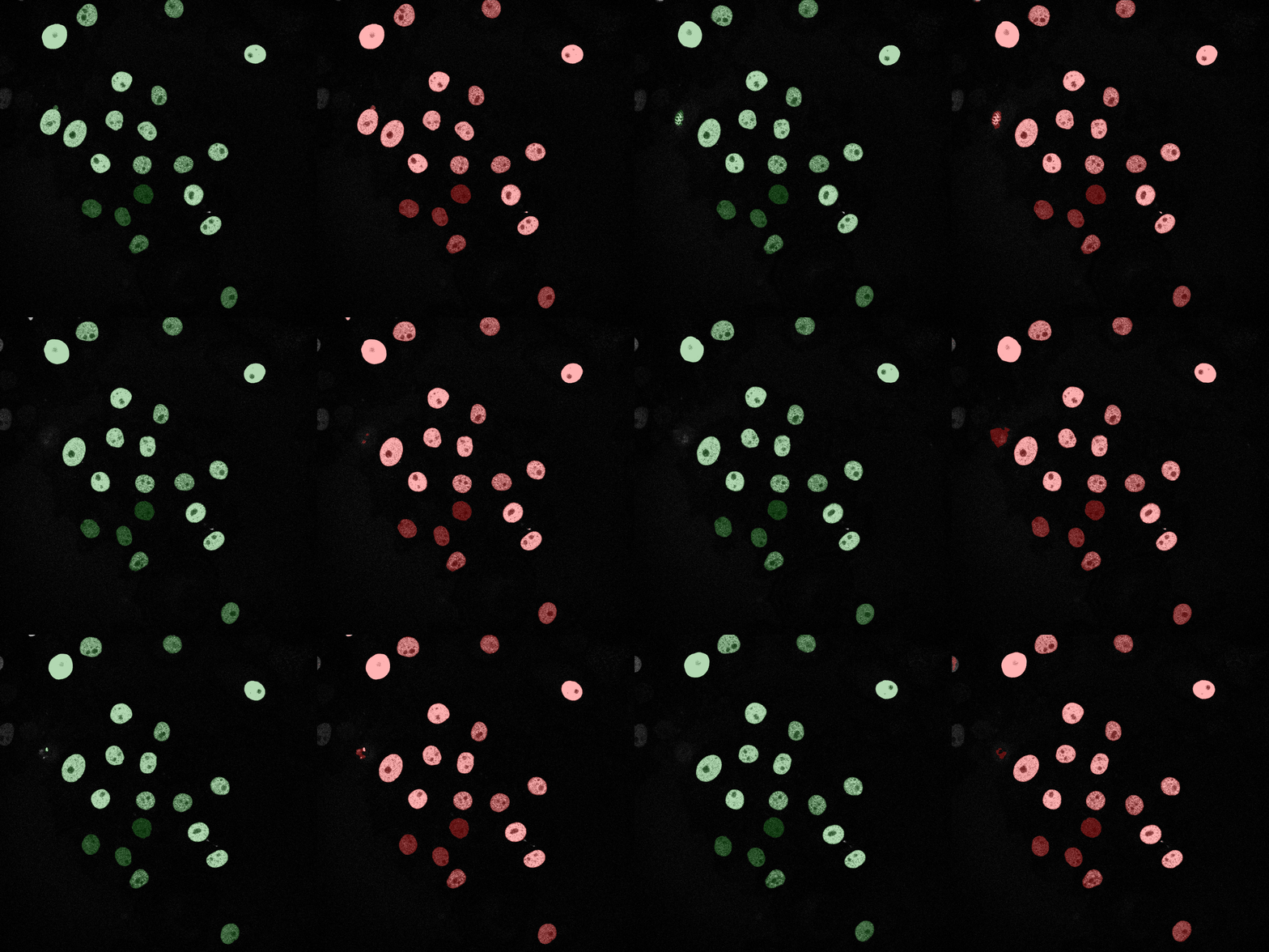
The U-Net model significantly outperforms all classical approaches, achieving a Mean IoU of 0.96 on Track 01 compared to the best classical model (MLP) at 0.91 and a Mean IoU of 0.93 on Track 02 compared to the best classical model at 0.87

Why U-Net is better:

1. Contextual Understanding: Classical models only see a tiny 5 × 5 patch around each pixel. They lack global context and cannot "see" the shape of the cell. U-Net processes the entire image at multiple scales, allowing it to understand cell morphology and separate cells from complex backgrounds.
2. Spatial Consistency: Pixel-wise classifiers treat every pixel independently, often resulting in "salt-and-pepper" noise where scattered pixels are misclassified. U-Net predicts a coherent mask, enforcing spatial continuity.
3. Feature Learning: Instead of relying on raw pixel intensities in a small window, U-Net learns hierarchical features (edges, textures, shapes) that are robust to noise and intensity variations common in microscopy images.

Tracking Results (Not Implemented)

Explain how you propagate identities across frames and highlight failure cases.

Demo Videos / GIFs

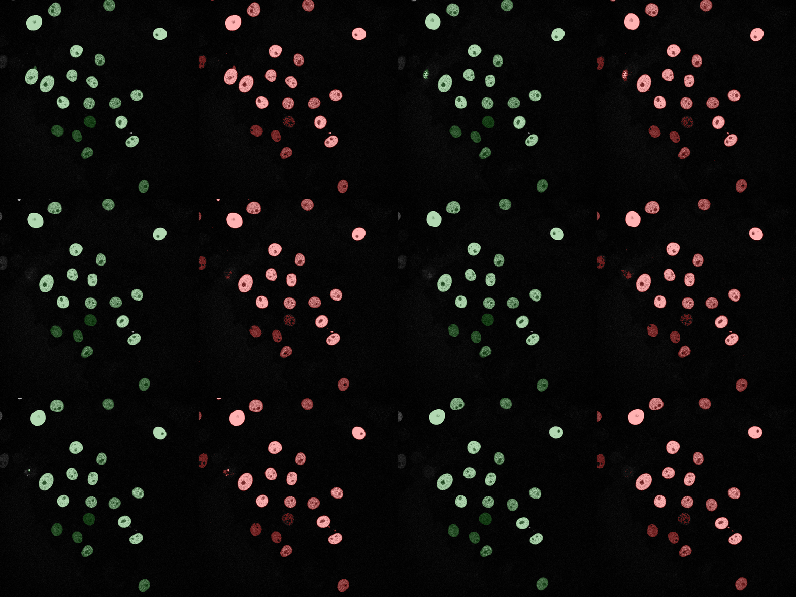
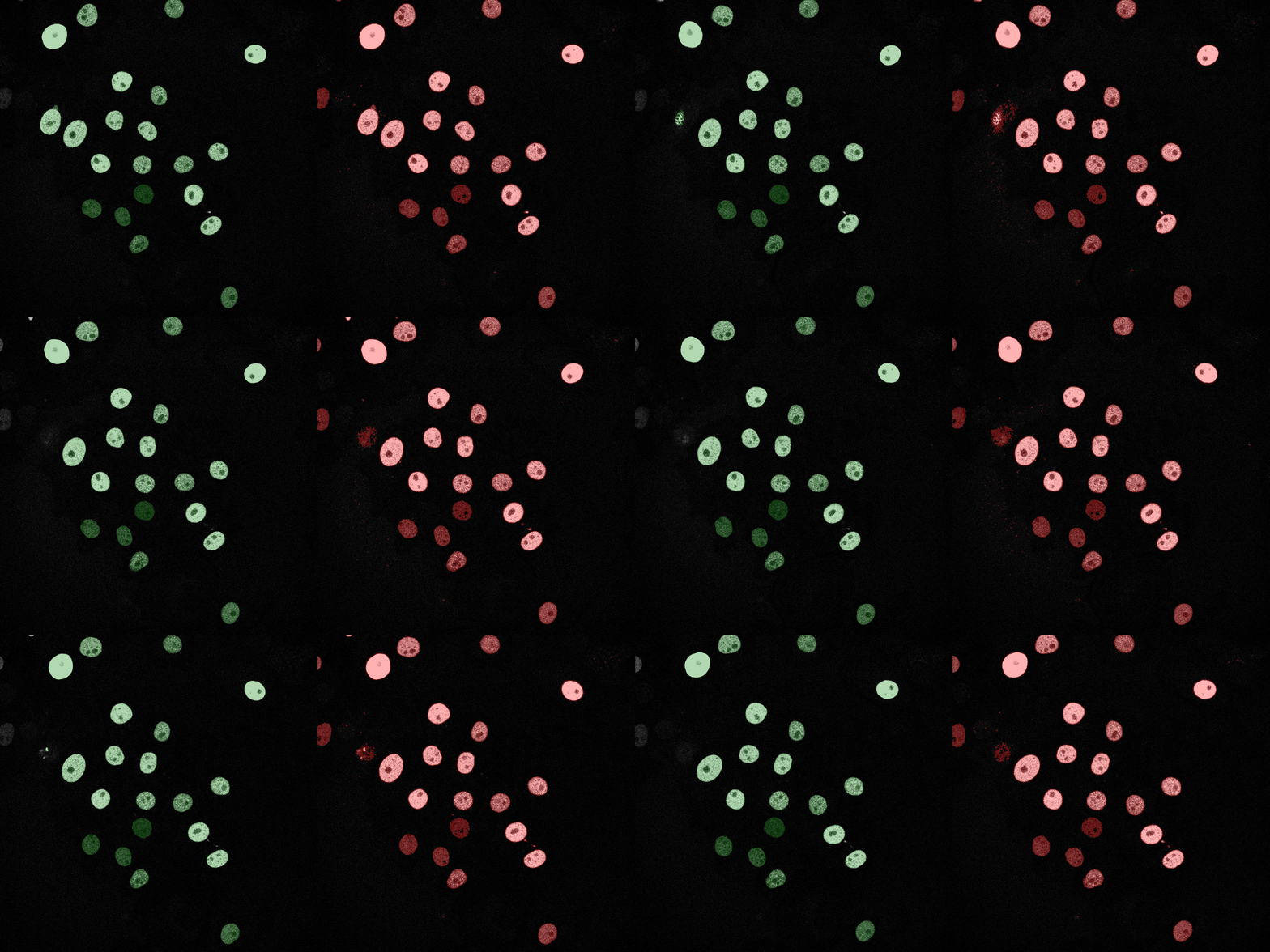
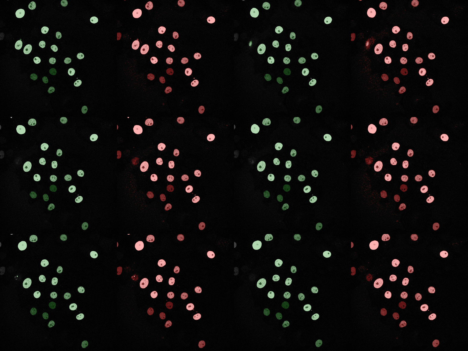
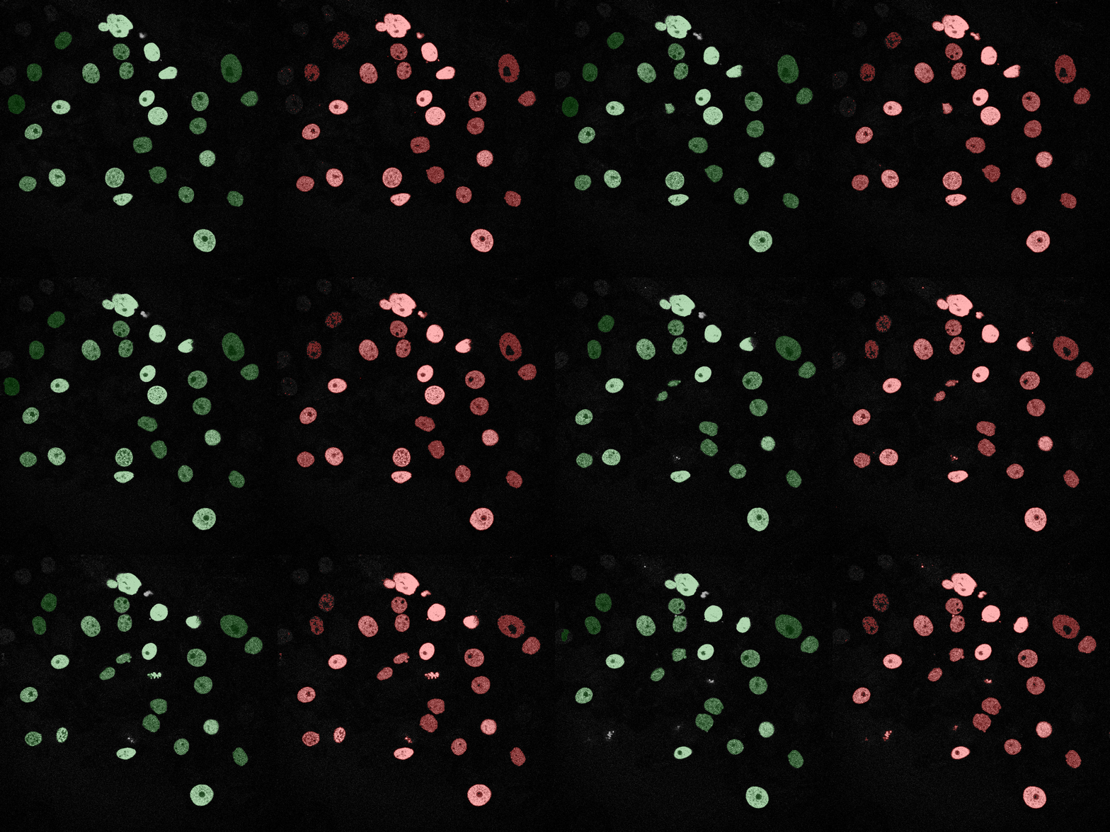
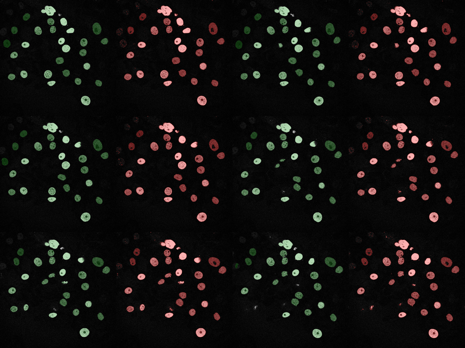
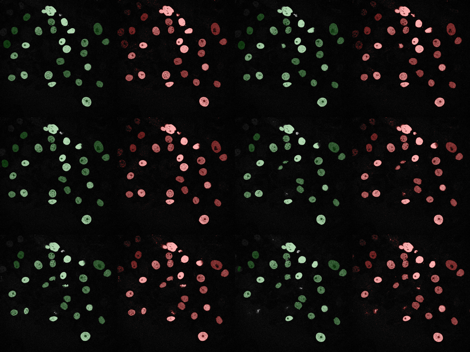
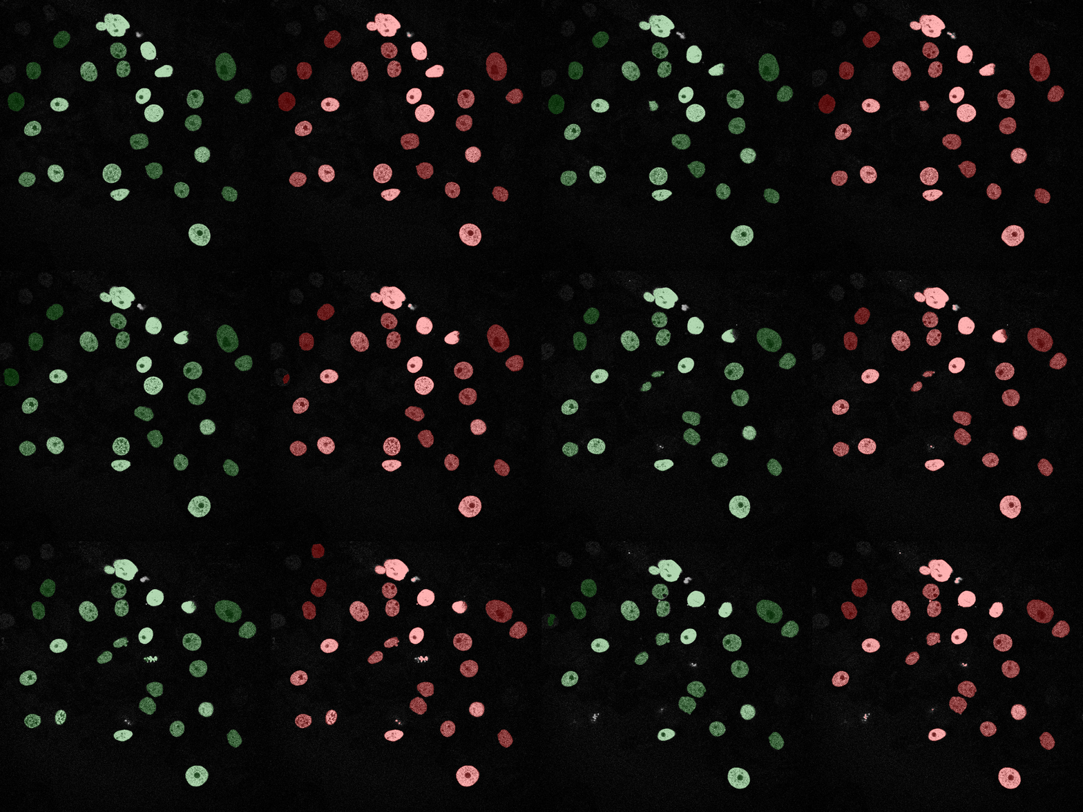
The following GIFs demonstrate the segmentation results on the validation set over time. For each figure, the left side shows the ground truth (Silver Truth) segmentation in green, while the right side shows the model's predicted segmentation in red.

Track 01

Naive Bayes

Linear SVM

SVM (RBF)

Logistic Regression

Neural Network (MLP)

U-Net (MobileNetV2)

Track 02

Naive Bayes

Linear SVM

SVM (RBF)

Logistic Regression

Neural Network (MLP)

U-Net (MobileNetV2)

Reproduction Checklist

To reproduce the results presented above, follow these steps:

1. Clone the Repository

git clone https://github.com/jfemiani/CSE488-Project-Cell-Tracking.git
cd CSE488-Project-Cell-Tracking

2. Environment Setup

Create a new Conda environment and install the required packages listed in pyproject.toml.

conda create -n cell-tracking python=3.11
conda activate cell-tracking
pip install -e .

Note: If you encounter build issues with albumentations on Windows, install a binary version explicitly:

pip install "albumentations==1.3.1"

3. Data Setup

Download and prepare the Fluo-N2DH-GOWT1 dataset with training/testing/validation

python scripts/setup_data.py --dataset Fluo-N2DH-GOWT1 --splits training test val

4. Train Classical Models

Train the baseline models (SVM, Naive Bayes, Logistic Regression, MLP) for both tracks.

# Train models for Track 01
python scripts/train_models.py --dataset Fluo-N2DH-GOWT1 --track 01 --window 5 --samples 500 --pct-fg 0.5

# Train models for Track 02
python scripts/train_models.py --dataset Fluo-N2DH-GOWT1 --track 02 --window 5 --samples 500 --pct-fg 0.5

5. Train U-Net Models

Train the deep learning U-Net models for both tracks.

# Train U-Net for Track 01
python scripts/train_unet.py --dataset Fluo-N2DH-GOWT1 --output-dir artifacts/models --track-id 01 --epochs 20

# Train U-Net for Track 02
python scripts/train_unet.py --dataset Fluo-N2DH-GOWT1 --output-dir artifacts/models --track-id 02 --epochs 20

6. Evaluate Segmentation

Evaluate all trained models (classical and deep learning) found in the artifacts/models directory. This script calculates the Mean IoU for each model, saves the results to artifacts/metrics, and saves resulted masked to artifacts/results

python scripts/eval_seg.py --dataset Fluo-N2DH-GOWT1 --models-dir artifacts/models

Full Artifacts Download

For full access to all trained models, segmentation results, and detailed metrics without running the reproduction scripts, you can download the compressed artifacts folder here:
Download Full Artifacts (Google Drive)

Lessons Learned / Next Steps

Share insights, what you'd try next, and open research questions.